I decided to structure this in phases. Day 1, everyone had to design some motion in their head and get it "checked off" by me as feasible. The basic requirements are that they need to have a wheel moving across space somehow, and they will eventually add a second point that rotates on the edge of this wheel. Day 1 went smoothly. Some of the kids had quite ambitious designs, so we came up with similar but simpler designs as backup options, in case there isn't enough time to do the whole shebang. They got on laptops and played around with the "Warm Up" portion of the packet, that gets them thinking about how to get a point MOVING in the plane as a function of t. I also asked them to try A = (cos(t), sin(t)) as a definition of a point, to see that it circles around (0, 0). They were delighted, but they understood why that works.
On Day 2, their goal was to get the center of the circle, point A, moving in the way that they had designed. So, just defining ONE point using parametric equations. I conferenced with each kid individually to help them get started, because some of their designs are quite tricky. Some kids figured it out entirely on their own. Once they figure it out, I ask them to use parametric equations to define a second point B, that will stay always a few units to the right of point A.
On Day 3, I thought this was a good check-in point, so I pulled the class together to talk about one person's equations for point A. It was something simple, like A = (2 + t, 4 + t). We talked about what the 2 and the 4 mean, and what the +t does to the coordinate values as t increases. We also talked about how you can get the point to move towards Quadrant III by changing the parametric equations, so that kids start to associate rates with parts of the equation. On Day 3, they created a circle from points A and B (using a circle tool built-in to GeoGebra -- we hadn't learned circular equations yet, and I just thought it was too many new concepts to throw into this project at once, especially because the circular equation is going to be parametrized as well). This is why we want B to remain "r" units to the right of point A; it makes it easy to then create the circle graphically, and it also helps to reinforce algebraically how do you translate the x coordinate without changing the y coordinate? Also on Day 3, I talked about how you would create a third point C = (cos(t), sin(t)) to simply rotate. But, how do we make it rotate around a bigger circle to match yours? How do we then modify it to rotate around a stagnant point such as (2, 3)? How do we then modify it to rotate around a dynamic point (2 + t, 4 + t)? If your kids are more adventurous than mine, they may be able to figure it all out on their own. Mine needed help with setting up the third point, but afterwards they were able to explain why this is done so.
On Days 4, 5, 6, kids were working on their written explanations of their 6 parametric equations; there are 2 parametric equations for point A (x(t) and y(t)), 2 parametric equations for point B, and 2 parametric equations for point C. They needed to write down explanations for every part of each equation, and explain how that part relates visually to the motion generated. They could also only explain the equations orally during their presentation, but then they would max out at 6/10 points for Communication, instead of potentially getting 10/10 points for both presenting orally and in writing. The explanations took them a long time to write, because I wanted them to do very detailed analysis involving all of these words: period, amplitude, midline, radius, independent variable, dependent variable, parametric equation. They also needed to present ONE interesting graph from among their 6 equations. If their graphs were not sufficiently interesting, they needed to go back and modify their design so that it would generate an interesting graph for our class discussion. Sometimes, this meant modifying the periods so that points A and C do not have the same period of movement.
Anyhow, here are SOME of my student samples. You can right-click on the t values and see the motion designed by my students! I'll talk about them here in more detail, so you can see what a wonderful variety of math concepts came out of this.
The translating wheel controlled by t1 was the first analysis we saw. The wheel simply translates in a linear path across the coordinate plane. The kid showed a graph of two functions that look like this:

Even though his design was relatively simple, he successfully explained with super clarity that one curve above shows the x-position of the rotating point C over time. It's cyclical, with an internal sub-period of 2pi because the equation is x(t) = 3cos(-t) + t, but its midline is no longer horizontal but a diagonal line with a positive slope, because the x-value of the center of the circle is increasing over time, thereby bringing C along with it to generally increase in x-value. He also explained that the second curve shows a downwards trend despite its cyclical nature, because generally the wheel is decreasing in position, so the y-coordinate of the rotating point will generally decrease over time despite the rotation around the circle.

Even though his design was simple, this student's presentation (which happened on Day 4) was a really good example for the rest of the kids, in terms of what level of detail they should incorporate and how to think about their equations. I think his classmates were really grateful that he went first to present, while they were still working on preparing their presentations and explanations, because he gave a really good blueprint to follow.
The rest are out of order for our presentations, but the "bounce" controlled by t2 generated an awesome graph from its rotating point's x-coordinate:

When the student presented this, we discussed it in the context of their algebraic equation for that point. x(t) = 2cos(t) + 2|cos(t)|. We talked about why the absolute-value was necessary as part of her point "A" (center of circle) to create the bounce, but also why that cancels out 2cos(t) for the parts of the period when cos(t) < 0. Lovely! Things that normally, my Precalc kids wouldn't see, arising naturally out of one of their creations.
 The planetary motion of t3 was interesting, because here the student was very deliberate about how long their periods were to be. One of the sub-periods in their design was 10, another was 20, and another was 30. The kid figured out that this meant that after 60 seconds, the whole system resets, which is visible inside the graph. (You can as well see the shorter internal periods.) I liked this presentation, because it helps to bring about the idea of periods within periods, and when does the system (if ever) reset?
I'll skip discussing t4 except to say that, how interesting it is that even though the motion here appears vastly different from the translating wheel in t1, their horizontal component movements are the same, and therefore their graphs for that component are also the same.
The "falling leaf" pattern controlled by t5 was massively interesting. The student only needed me to ask him guiding questions through the baby steps of first setting it up such that it's falling straight down (something like (4, 5 - t), then additionally falling left-and-right, something like (cos(t), 5 - t). After that, he was ready to make it entirely his own. His final parametric equations for the falling center looked like this: (t^1.1 cos(t), 20 - 1.2^t). The t^1.1 part, he explained, means that his amplitude of falling left-and-right increases as t increases. He also explained to the class that the 1.2^t means that as t increases, the leaf falls exponentially faster and faster in the vertical direction. This he came up with entirely on his own, by playing around with possibilities of varying the equation! That's amazing. He said that a falling leaf should fall more and more sideways, and faster and faster vertically.
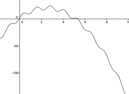
The rotating point for this wheel has a y(t) graph that looks like this (see below). The equation is y(t) = 2sin(t + 2) + 20 - 1.2^t. This student explained that the period of rotation of 2sin(t + 2) is still 2pi, but the "falling leaf" circle starts to drop so fast vertically, that the rotating period doesn't really matter after a little while. After about 10 seconds, the effect of the rotation on the height of that point isn't really visible compared to the overall exponential movement of the wheel.

The parabolic motion controlled by t6 is interesting, because I had to work with the kid to remind him how to do parabolic analysis. He wanted a parabola that would turn around after going up for a while, so we wanted a parabola whose vertex has a positive t value. The student still remembered -b/(2a) for the axis of symmetry equation, so I helped him make the connection that if he wanted a downwards parabola (which he remembered that means a < 0), then b > 0 would cause a positive t-value for the vertex. He then played around with it and decided that a = -3 and b = 15 were good values to use. To help him separate the ideas of t and x(t), I asked him to figure out how to make his wheel go LEFT as it rises and falls. He did well with this, and he was also able to explain why the height of the rotating point gets overwhelmed by the general parabolic change of height. He even explained that normally, t = -15/-6 = 2.5 seconds would be the max height, but here since the rotation changes the shape of the graph we're examining, the max will occur around 2.5 seconds but not then exactly.
Lastly, the wheel that resembles a swinging pendulum was pretty complex to create. I had to help the student create the up-down motion after they created the left-right motion, because the up-down motion has a period that is half of the left-right motion, and also their phase shifts should match up. (For every time that the pendulum goes all the way right and back to the left, that's one full horizontal period ending at t = 2pi. But, in that time its vertical motion has already completed two full periods, hitting the max at t = pi and t = 2pi.) That's a bit tricky for the kids, but I liked the reminder that the pendulum motion has related but different periods for vertical and horizontal components, since it was something that we had briefly discussed a long time ago.
The graph that was generated from the horizontal position of the rotating point C looked like this:

Overall, this project was definitely challenging, but I thought that it really stretched their understanding of the forms of functions. It was also a great way to tie in math to something real. I told them that for making animated movies, people obviously don't manually put in every coordinate of the object for every fraction of a second. A lot of it is controlled by parametrized movements and automated calculations as a function of t!
No comments:
Post a Comment